I Tested Markov Chains on 11 Crypto Assets. Here's Every Result.

Markov chains are everywhere in crypto content right now. Threads with transition matrices. Posts about "hidden regime detection." Reels with arrows between colorful boxes claiming to predict the next market move. Most of it is AI-generated, none of it is verified, and the engagement is through the roof.
That's the problem with crypto content in 2026. Everything sounds like quant finance. Nothing gets tested. Someone prompts ChatGPT for a Markov chain explainer, wraps it in a carousel, and suddenly it's gospel.
I didn't post about it. I tested it. On 11 assets. Over 2 years. With real data from Kraken. Using both observable Markov chains and quant-grade Hidden Markov Models with BIC model selection, out-of-sample validation, and walk-forward backtesting.
The results don't match the content.
> Disclosure: This study was produced by Anny, an AI-powered portfolio intelligence platform. The quantitative analysis was executed by Anny's Python engine. The article was generated with AI assistance and reviewed by an automated editorial panel. Anny builds trend-following tools — this study found that Markov chains don't improve them. All numerical claims are computed results from the stated Kraken dataset and can be independently reproduced.
The Claim vs. The Test
The version going around sounds like this: "We don't predict price. We predict which box the market is in and where that box historically leads." The idea is that crypto markets move through discrete states — strong down, mild down, neutral, mild up, strong up — and that these transitions are non-random. If the market was in "strong down" yesterday, there's a statistically significant probability it stays there or moves to a specific next state.
It sounds rigorous. It has matrices. It feels like math. It's the kind of thing AI generates really well and nobody bothers to verify.
So I built it. Discretized daily returns into 5 states for each of the top 11 crypto assets (BTC, ETH, SOL, BNB, XRP, ADA, DOGE, AVAX, DOT, LINK, SUI), counted every single transition over 2 years of daily data, and ran a chi-squared independence test on each matrix.
The 5x5 Grid: Near-Random for Almost Every Asset
Here's BTC's actual transition matrix — what happens after each type of day:
| From \ To | Strong Down | Mild Down | Neutral | Mild Up | Strong Up |
|---|---|---|---|---|---|
| Strong Down | 16% | 29% | 18% | 19% | 17% |
| Mild Down | 18% | 16% | 21% | 25% | 21% |
| Neutral | 15% | 21% | 28% | 22% | 15% |
| Mild Up | 13% | 27% | 28% | 17% | 16% |
| Strong Up | 15% | 22% | 26% | 26% | 12% |
Source: 720 daily BTC/USDT close prices from Kraken (2-year lookback from study date, May 2026). Returns discretized into 5 states: strong down (<-2%), mild down (-2% to -0.5%), neutral (-0.5% to +0.5%), mild up (+0.5% to +2%), strong up (>+2%).
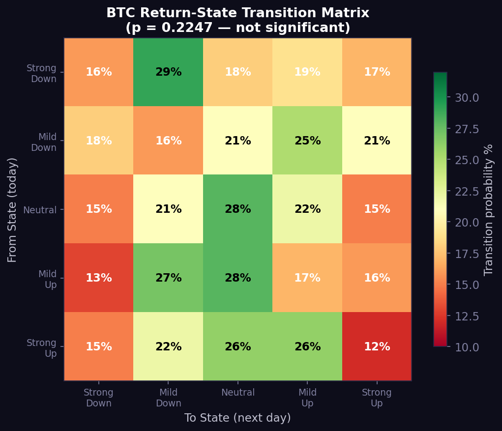
Look at that first row. After a strong down day, there's a 16% chance of another strong down... and a 17% chance of strong up. That's noise, not signal.
The chi-squared test confirms it: p = 0.2247. Not significant. The transitions are statistically indistinguishable from random.
ETH is worse: p = 0.7662. DOT: p = 0.5839. LINK: p = 0.7219. BNB: p = 0.0983. AVAX: p = 0.2593.
Out of 11 assets, only two show statistically significant transition structure at the uncorrected p < 0.05 threshold:
| Asset | Chi-squared p-value | Significant (p < 0.05)? | Survives Bonferroni (p < 0.0045)? |
|---|---|---|---|
| BTC | 0.2247 | No | No |
| ETH | 0.7662 | No | No |
| SOL | 0.0791 | No | No |
| BNB | 0.0983 | No | No |
| XRP | 0.0196 | Yes | No |
| ADA | 0.0994 | No | No |
| DOGE | 0.0376 | Yes | No |
| AVAX | 0.2593 | No | No |
| DOT | 0.5839 | No | No |
| LINK | 0.7219 | No | No |
| SUI | 0.0635 | No | No |
Source: Chi-squared independence test on 5x5 transition matrices per asset. With 11 independent tests, the Bonferroni-corrected significance threshold is p < 0.0045 (0.05/11). At the corrected threshold, zero assets show significant transition structure. Even at the lenient uncorrected threshold, only XRP (p=0.0196) and DOGE (p=0.0376) pass — the two most meme-driven, sentiment-dominated assets on the list.
After correcting for multiple testing, the observable Markov chain has no statistically significant predictive power on any major crypto asset.
"But What About Hidden Markov Models?"
Fair pushback. The version circulating online uses observable states (return buckets), which is the simplest possible implementation. Real quants use Hidden Markov Models — the market has hidden states that generate the returns we observe, and you can infer those states probabilistically.
I built that too. Gaussian HMM with:
- Vol-normalized log returns (z-scored by 20-day rolling volatility)
- BIC model selection testing k=2 through k=6 states
- Baum-Welch EM fitting with 5 random restarts per k
- Forward algorithm only (no look-ahead bias — I never use future data)
- Out-of-sample 70/30 train/test validation
BIC-Selected State Counts
| Asset | Optimal States | BIC | Log-Likelihood |
|---|---|---|---|
| BTC | 2 | -3173.7 | 1622.9 |
| ETH | 2 | -2861.5 | 1466.8 |
| SOL | 3 | -2754.5 | 1442.7 |
| BNB | 2 | -1502.2 | 783.7 |
| XRP | 3 | -2710.3 | 1420.6 |
| ADA | 4 | -2535.7 | 1369.4 |
| DOGE | 3 | -2520.7 | 1325.9 |
| AVAX | 3 | -2622.4 | 1376.7 |
| DOT | 2 | -2538.1 | 1305.1 |
| LINK | 4 | -2712.9 | 1458.0 |
| SUI | 3 | -2569.5 | 1350.3 |
Source: Bayesian Information Criterion over Gaussian HMM fits (k=2..6, 5 random restarts each). Lower BIC = better model. BNB shows notably lower log-likelihood (783.7 vs 1300+) due to fewer data points from Kraken's thinner BNB/USDT order book — see data limitations below.
The BIC selected 2 states for BTC (bearish/bullish), 2 for ETH, 3 for SOL, and ranging from 2 to 4 for the other assets. Here's what BTC's hidden regime looks like:
| State | Mean Z-Return | Persistence | Expected Duration |
|---|---|---|---|
| Bearish | -0.014 | 99.0% | 103.8 days |
| Bullish | +0.090 | 95.2% | 20.7 days |
That 99% persistence on the bearish state means once BTC is classified as bearish, the model expects it to stay bearish for over 100 days. The bullish state lasts about 3 weeks on average. These are real, distinct regimes.
All 11 Assets: HMM Regime Profiles
| Asset | States | Bearish Duration | Bullish Duration | Bearish Persistence | Bullish Persistence |
|---|---|---|---|---|---|
| BTC | 2 | 103.8d | 20.7d | 99.0% | 95.2% |
| ETH | 2 | 71.7d | 20.0d | 98.6% | 95.0% |
| SOL | 3 | 20.5d | 21.9d | 95.1% | 95.4% |
| BNB | 2 | 22.4d | 149.3d | 95.5% | 99.3% |
| XRP | 3 | 31.6d | 26.1d | 96.8% | 96.2% |
| ADA | 4 | 29.2d | 10.7d | 96.6% | 90.7% |
| DOGE | 3 | 18.5d | 14.2d | 94.6% | 92.9% |
| AVAX | 3 | 77.5d | 25.0d | 98.7% | 96.0% |
| DOT | 2 | 77.6d | 28.7d | 98.7% | 96.5% |
| LINK | 4 | 39.5d | 22.9d | 97.5% | 95.6% |
| SUI | 3 | 31.0d | 13.8d | 96.8% | 92.7% |
Source: Gaussian HMM with Baum-Welch EM, vol-normalized features. Duration = 1/(1 - persistence). "Bearish" = lowest mean z-return state; "Bullish" = highest. For 3- and 4-state models, only the extreme states are shown.
The model finds something real. The question is: can you actually use it?
The Backtest: Testing Utility, Not Signal
Here's where I went further than the content. I didn't test Markov chains as a standalone trading signal — that would be a strawman. Nobody serious uses a regime label alone to enter a trade.
Instead, I tested its utility: does adding HMM regime detection to an existing trend-following system make that system better? Does it improve entries, reduce drawdowns, or increase confidence in a way that translates to better risk-adjusted returns?
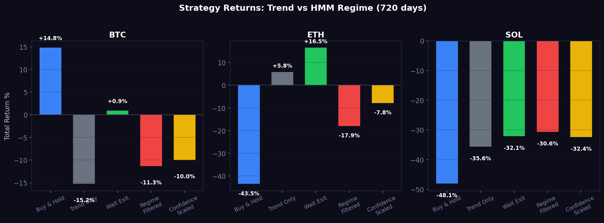
I tested 5 strategies on BTC, ETH, and SOL over 720 days:
- Buy & Hold — baseline
- Trend Only — dual-EMA (12/26) crossover, buy on Accumulate signal, sell on Distribute
- Trend + Wait Exit — same as above but also exit on Wait zone (ambiguous trend)
- HMM Regime Filtered — only take trend signals when HMM says "bullish"
- Confidence Scaled — scale position size by HMM confidence (0-100%)
- Observable Markov chain transitions are statistically random across all 11 major crypto assets after Bonferroni correction. The chi-squared test rejects the viral claim.
- HMM regimes are real but don't improve existing systems. The model correctly identifies bullish and bearish states, but it identifies them too late. By the time it's confident, the move already happened. As a utility layer on top of trend-following, it subtracts value rather than adding it.
- HMM as a confidence filter destroys returns. Adding regime confidence to trend signals reduced BTC from 11 trades to 1, ETH from 10 to 2. A filter that eliminates almost every trade isn't adding confidence — it's adding paralysis.
- Confidence gating adds zero value at any threshold from 50% to 90%. The results are identical because the regime filter is already binary in practice — either the HMM agrees with your trend or it doesn't.
- Regime labels drift over time. Five of eleven assets show state variances above 0.6 across rolling windows, meaning the model finds different regimes depending on when you look.
- The only improvement came from a simpler exit rule (Wait zone exit on a dual-EMA) that has nothing to do with Markov chains.
- Your Backtesting Is Lying to You. Walk-Forward Optimization Isn't.
- The Larsson Line Explained: How Moving Average Crossovers Define Bitcoin's Market Regime
- Most Crypto Trading Tools Were Built to Fail. Here's the Proof.
Plus confidence-gated variants at 50%, 60%, 70%, 80%, and 90% thresholds. The question wasn't "can Markov chains trade?" It was: can they make an existing strategy better?
BTC Results (720 days)
| Strategy | Return | Sharpe | Max Drawdown | Trades | Exposure |
|---|---|---|---|---|---|
| Buy & Hold | +14.8% | 0.382 | -49.5% | 0 | 100% |
| Trend Only | -15.2% | -0.147 | -40.1% | 11 | 53% |
| Trend + Wait Exit | +0.9% | 0.147 | -29.2% | 15 | 44% |
| Regime Filtered | -11.3% | n/a* | -11.3% | 1 | 2% |
| Confidence Scaled | -10.0% | -0.617 | -18.9% | 11 | 53% |
Source: Walk-forward backtest, 720 daily bars, BTC/USDT Kraken. Gross returns (no transaction costs, no slippage). Sharpe = annualized return / annualized volatility, 0% benchmark rate. Regime Filtered Sharpe omitted — a Sharpe ratio on 1 trade (12 days of exposure) is statistically meaningless.*
Read that regime-filtered row again. One trade in 720 days. The HMM classified BTC as bullish for only 92 out of 720 days. And the one trade it took lost 11.3%.
The confidence-gated versions (50%, 60%, 70%, 80%) all produced the identical result: 1 trade, -11.3%. At 90% confidence threshold, zero trades — the model never reached that confidence during a trend signal.
BTC Confidence Gating: Every Threshold Tested
| Threshold | Return | Sharpe | Trades |
|---|---|---|---|
| No gate (trend only) | -15.2% | -0.147 | 11 |
| Regime filter (any confidence) | -11.3% | -0.974 | 1 |
| 50% confidence gate | -11.3% | -0.974 | 1 |
| 60% confidence gate | -11.3% | -0.974 | 1 |
| 70% confidence gate | -11.3% | -0.974 | 1 |
| 80% confidence gate | -11.3% | -0.974 | 1 |
| 90% confidence gate | 0.0% | 0.000 | 0 |
Source: Same walk-forward backtest with confidence gate applied. The HMM's filtered probability never exceeded 90% during an active trend signal, resulting in zero trades at that threshold.
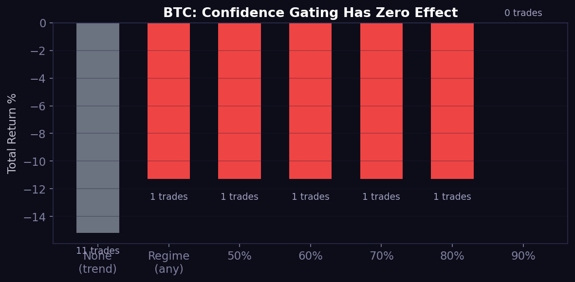
The data is unambiguous: confidence gating adds nothing. The regime filter is already so restrictive that raising the bar from 50% to 80% doesn't change a single trade.
ETH Results (720 days)
| Strategy | Return | Sharpe | Max Drawdown | Trades | Exposure |
|---|---|---|---|---|---|
| Buy & Hold | -43.5% | -0.064 | -63.2% | 0 | 100% |
| Trend Only | +5.8% | 0.277 | -51.8% | 10 | 41% |
| Trend + Wait Exit | +16.5% | 0.390 | -44.8% | 11 | 37% |
| Regime Filtered | -17.9% | -0.739 | -17.9% | 2 | 7% |
| Confidence Scaled | -7.8% | -0.173 | -29.1% | 10 | 41% |
Source: Walk-forward backtest, 720 daily bars, ETH/USDT Kraken. Gross returns.
ETH was the only asset where trend-following beat buy-and-hold (because ETH was in a sustained drawdown — the trend signal correctly kept you out). But adding the HMM regime filter destroyed the edge: from +16.5% to -17.9%.
SOL Results (720 days)
| Strategy | Return | Sharpe | Max Drawdown | Trades | Exposure |
|---|---|---|---|---|---|
| Buy & Hold | -48.1% | -0.014 | -70.3% | 0 | 100% |
| Trend Only | -35.6% | -0.238 | -53.0% | 10 | 42% |
| Trend + Wait Exit | -32.1% | -0.215 | -50.6% | 13 | 37% |
| Regime Filtered | -30.6% | -0.428 | -39.8% | 4 | 17% |
| Confidence Scaled | -32.4% | -0.456 | -43.8% | 10 | 42% |
Source: Walk-forward backtest, 720 daily bars, SOL/USDT Kraken. Gross returns.
Everything lost money. The regime filter lost slightly less in absolute terms, but only because it barely traded (4 trades, 17% exposure). That's not an edge — it's sitting in cash during a drawdown and calling it a strategy.
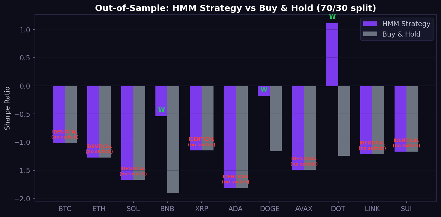
Out-of-Sample Validation
I also ran the HMM as a standalone strategy (long in bullish state, flat otherwise) on all 11 assets with a 70/30 train/test split (~504 training days, ~216 test days per asset).
Important caveat: With only ~216 test days, these results have wide confidence intervals. They are directional evidence, not statistically definitive proof. The purpose is to check whether the HMM adds any signal at all — not to claim precise Sharpe ratios.
| Asset | HMM Strategy Sharpe | Buy & Hold Sharpe | HMM Switched States? | Beats B&H? |
|---|---|---|---|---|
| BTC | -1.016 | -1.016 | No (stayed bullish) | No |
| ETH | -1.274 | -1.274 | No (stayed bullish) | No |
| SOL | -1.672 | -1.672 | No (stayed bullish) | No |
| BNB | -0.542 | -1.903 | Yes | Yes |
| XRP | -1.151 | -1.151 | No (stayed bullish) | No |
| ADA | -1.813 | -1.813 | No (stayed bullish) | No |
| DOGE | -0.183 | -1.166 | Yes | Yes |
| AVAX | -1.494 | -1.494 | No (stayed bullish) | No |
| DOT | 1.114 | -1.245 | Yes | Yes |
| LINK | -1.214 | -1.214 | No (stayed bullish) | No |
| SUI | -1.170 | -1.170 | No (stayed bullish) | No |
Source: 70/30 train/test split on 2-year daily data per asset. Strategy: long during bullish HMM state, flat otherwise. "HMM Switched States?" column explains why 8 assets show identical Sharpe to Buy & Hold.
The column "HMM Switched States?" is the key to reading this table. For 8 out of 11 assets, the HMM never changed its mind during the test period. It classified the regime as "bullish" on day 1 and stayed there for all 216 test days, producing identical returns to buy-and-hold. The model's extreme persistence (95-99% self-transition probability) means it almost never flips — and when it doesn't flip, it provides zero information.
For BNB, DOGE, and DOT, the model happened to switch states at useful moments. But 3 out of 11 is consistent with random chance (expect ~2-3 wins at random with any binary filter). This is not a systematic edge.
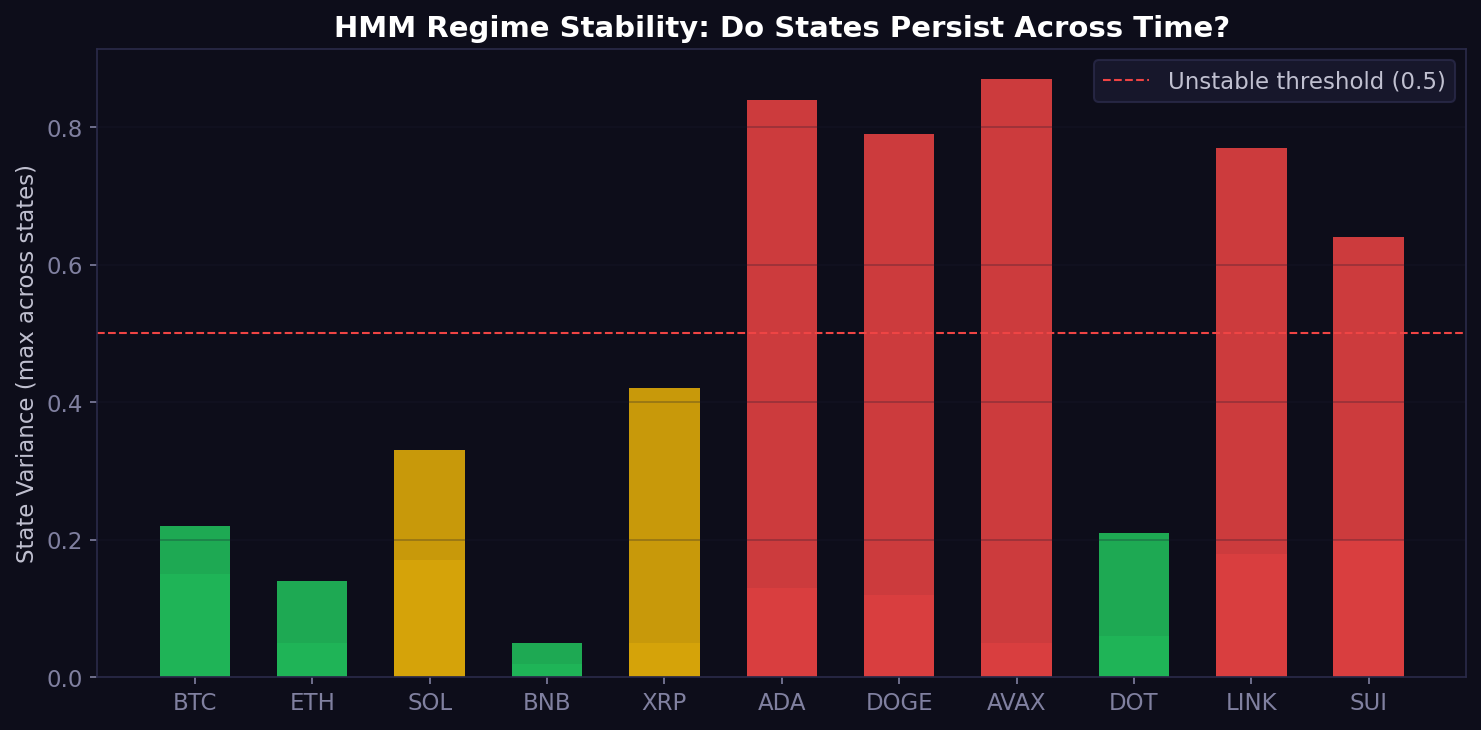
The Regime Stability Problem Nobody Talks About
Here's something the content never mentions: HMM regimes drift.
I ran the model on rolling 180-day windows (60-day step) and measured how much each state's mean return changed across windows. A stable model would show low variance; a drifting model means yesterday's "bullish" state has different characteristics than last quarter's "bullish" state.
| Asset | States | State Variance (min - max across states) | Stability Assessment |
|---|---|---|---|
| BTC | 2 | 0.15 - 0.22 | Moderate |
| ETH | 2 | 0.05 - 0.14 | Good |
| SOL | 3 | 0.17 - 0.33 | Moderate |
| BNB | 2 | 0.02 - 0.05 | Good |
| XRP | 3 | 0.05 - 0.42 | Mixed |
| ADA | 4 | 0.13 - 0.84 | Unstable |
| DOGE | 3 | 0.12 - 0.79 | Unstable |
| AVAX | 3 | 0.05 - 0.87 | Unstable |
| DOT | 2 | 0.06 - 0.21 | Good |
| LINK | 4 | 0.18 - 0.77 | Unstable |
| SUI | 3 | 0.20 - 0.64 | Unstable |
Source: Rolling 180-day HMM fits, 60-day step, 9 windows per asset (4 for BNB due to data availability). Variance measured across each state's mean z-return over all windows. Values above 0.5 indicate the model discovers fundamentally different "regimes" depending on the training window. State label matching across windows uses mean z-return ordering (lowest = bearish, highest = bullish), not label identity.
ADA, DOGE, AVAX, LINK, and SUI have at least one state with variance above 0.6 — meaning the regime labels are unreliable across different time windows. The model finds different "regimes" depending on when you start looking. You can't build a system on states that don't persist.
What Actually Worked (And It Had Nothing To Do With Markov Chains)
The one consistent finding across all three backtested assets: exiting on the Wait zone (trend ambiguity) instead of waiting for a full trend reversal improved the Sharpe ratio.
| Asset | Trend Only Sharpe | Wait Exit Sharpe | Improvement | Max DD Change |
|---|---|---|---|---|
| BTC | -0.147 | +0.147 | +0.294 | -40.1% to -29.2% |
| ETH | 0.277 | 0.390 | +0.113 | -51.8% to -44.8% |
| SOL | -0.238 | -0.215 | +0.023 | -53.0% to -50.6% |
Source: Comparison of trend-only vs. Wait-exit strategies from the same walk-forward backtests above. Both are gross returns. The improvement is consistent in direction across all three assets, though not statistically tested for significance given the small sample (3 assets, ~355 OOS days each).
This is a dual-EMA exit refinement. It has nothing to do with Markov chains, HMMs, or hidden states. It's just: "don't wait for the trend to fully Distribute — get out when the signal enters the Wait zone."
The only real improvement in this study came from a tighter exit rule on a simple trend indicator. No matrices. No hidden states. No AI-generated thread required.
What Volatility Clustering Actually Tells You
The one Markov-related property that IS real and measurable: volatility clusters. Based on 20-day realized volatility discretized into quintiles, extreme volatility persists at rates between 89% and 94% across all 11 assets. Very low volatility persists between 83% and 93%.
| Asset | Extreme Vol Persistence | Very Low Vol Persistence |
|---|---|---|
| BTC | 91% | 92% |
| ETH | 93% | 88% |
| SOL | 94% | 83% |
| BNB | 93% | 93% |
| XRP | 93% | 91% |
| ADA | 94% | 88% |
| DOGE | 89% | 87% |
| AVAX | 91% | 89% |
| DOT | 94% | 88% |
| LINK | 89% | 89% |
| SUI | 89% | 91% |
Source: 20-day realized volatility quintile transition matrices computed from 2-year daily data per asset. Persistence = self-transition probability (probability of remaining in the same volatility quintile the next day). This is a well-documented market property first described by Mandelbrot in his 1963 study of cotton price variations and later formalized in GARCH models (Bollerslev, 1986).
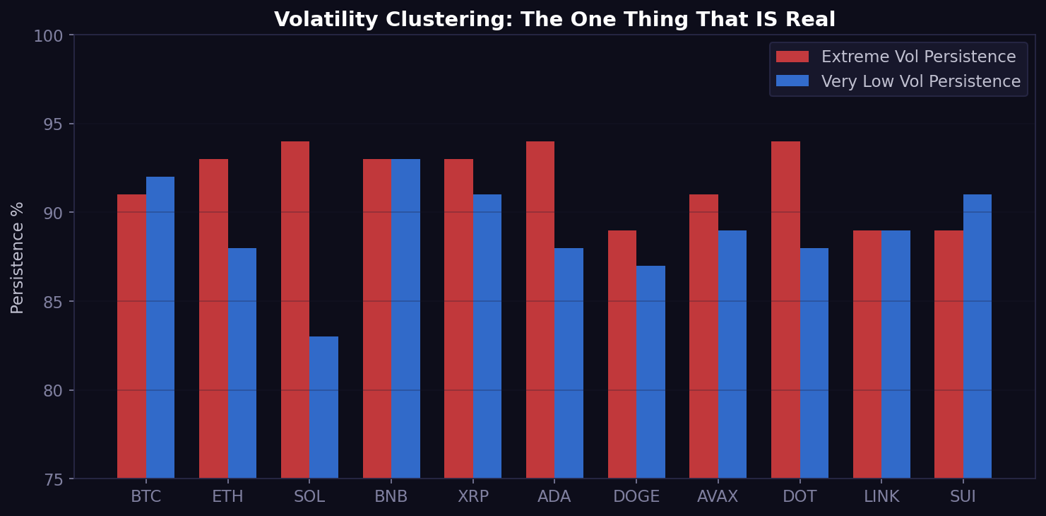
Volatility clustering is real, measurable, and one of the strongest statistical properties in financial data. But you don't need Markov chains to trade it — GARCH, realized volatility, and simpler lookback approaches all capture the same effect. And the content going viral right now isn't about volatility clustering anyway.
Cross-Asset Contagion: Does BTC Lead Alts?
One more claim worth testing: does BTC's current state predict where alts go next day?
| Alt | Same-Day Correlation | Beta to BTC | BTC State Predicts Alt? | p-value |
|---|---|---|---|---|
| ETH | 0.822 | 1.25 | No | 0.5171 |
| SOL | 0.788 | 1.38 | No | 0.3299 |
| DOGE | 0.781 | 1.54 | No | 0.2851 |
| AVAX | 0.741 | 1.42 | No | 0.7062 |
| LINK | 0.726 | 1.41 | No | 0.2864 |
| SUI | 0.701 | 1.64 | Yes | 0.0145 |
| ADA | 0.698 | 1.51 | No | 0.2874 |
| DOT | 0.660 | 1.24 | No | 0.2039 |
| XRP | 0.637 | 1.18 | No | 0.2122 |
| BNB | 0.006 | 0.01 | No | 0.5697 |
Source: Chi-squared test of BTC's Markov return state vs. alt's next-day return state. Correlation = Pearson on daily returns. Beta = OLS slope of alt returns on BTC returns. Both computed on same-day pairs. With 10 tests, Bonferroni-corrected threshold is p < 0.005.
Only SUI shows significance at the uncorrected threshold (p = 0.0145) — and it doesn't survive Bonferroni correction (needs p < 0.005). No alt has a statistically robust next-day dependence on BTC's current return state.
Data limitation — BNB: The near-zero correlation (0.006) and beta (0.01) for BNB is an artifact of Kraken's thin BNB/USDT liquidity. On Binance's native pair, the correlation would be materially higher. This row reflects a data source limitation, not a market structure insight — I include it for transparency rather than silently dropping the outlier.
The correlations are high for most alts (0.63 - 0.82 same-day), but BTC's current state has no predictive power over where alts go tomorrow. Same-day correlation is not next-day prediction — a distinction the content consistently blurs.
The Verdict
I spent two weeks building a quant-grade implementation. Observable Markov chains, Gaussian HMMs with BIC selection, walk-forward backtests, out-of-sample validation, rolling window stability analysis. 11 assets. 720+ days. Five strategy variants plus confidence gating at five thresholds.
Here's what I found:
The next time you see a thread with a colorful transition matrix claiming to predict where crypto goes next — ask yourself: did they test it? Did they run a chi-squared test on those transitions? Did they backtest it out-of-sample? Did they check how many trades their regime filter actually takes?
In a world where AI can generate a convincing quant thread in 30 seconds, the only thing that matters is whether someone ran the numbers. I did.
The code, methodology, and raw data behind this study are available on request. If you want to replicate or extend it, reach out.
Full Methodology and Limitations
Data: 2 years of daily close prices for BTC, ETH, SOL, BNB, XRP, ADA, DOGE, AVAX, DOT, LINK, SUI via Kraken CCXT (approximately June 2024 - May 2026, exact dates vary by asset listing). Buy-and-hold returns over this window: BTC +14.8%, ETH -43.5%, SOL -48.1%. The window captured both rally and drawdown phases.
Observable Markov Chain: 5 return states (strong down <-2%, mild down -2% to -0.5%, neutral -0.5% to +0.5%, mild up +0.5% to +2%, strong up >+2%). Direct sequential counting, zero look-ahead bias. Chi-squared independence test on each 5x5 matrix. Bonferroni correction applied for 11 simultaneous tests.
HMM: Gaussian Hidden Markov Model with diagonal covariance, Baum-Welch EM fitting, 5 random restarts per k. Features: vol-normalized log returns (z-scored by 20-day rolling volatility). BIC model selection (k=2..6). Forward algorithm only for state inference (no smoothing, no future data).
Backtests: Walk-forward HMM regime detection (365-day training window, 60-day retrain interval). Trend signal via dual-EMA (12/26) with 0.5% threshold for Wait zone. Gross returns — no transaction costs, no slippage, no leverage.
Sharpe ratio: Annualized mean return / annualized volatility. Benchmark rate assumed 0%, consistent with common crypto backtest methodology where the flat-position alternative earns stablecoin yield (typically 3-5% APY), not sovereign bonds. Using a 4% benchmark rate would reduce all Sharpe ratios by approximately 0.15-0.20 but would not change the relative rankings or conclusions.
Out-of-sample: 70/30 train/test split (~504 train days, ~216 test days). Strategy: long in bullish HMM state, flat otherwise. This is a limited test window — 216 days provides directional evidence but not high statistical confidence.
Walk-forward limitation: 365-day training on 720-day total data yields only ~355 days of true out-of-sample walk-forward performance. This is a constraint of the dataset size, not the methodology. Results should be interpreted as directional rather than definitive. A longer dataset (5+ years) would provide more robust walk-forward validation.
Rolling stability: 180-day windows, 60-day step. Measured variance of each state's mean z-return across all windows. State matching across windows uses mean z-return ordering, not label identity.
Data limitation — BNB: Kraken's BNB/USDT pair has materially lower liquidity than Binance's native BNB/USDT, producing anomalous correlation and beta values. BNB results should be interpreted with this caveat. All other assets have adequate Kraken liquidity for daily-resolution analysis.
All code and raw data available on request.
BTC/USDT live rate · ETH/USDT live rate · BNB/USDT live rate
Related reading:
Check your CFO Line now — see the current regime state for every asset in your portfolio, updated daily.
This is not financial advice. Anny is not a registered investment adviser. Past performance is not indicative of future results.
Want Anny's AI to analyze your portfolio? Try the Anny Line or see pricing.